Welcome to R!
Last updated on 2025-04-15 | Edit this page
Estimated time: 180 minutes
Overview
Questions
- Why bother learning R?
- What is RStudio? Why use it instead of “base R?”
- What am I looking at when I open RStudio?
- How do I “talk to” R and ask it to do things?
- What things can I make R build? What things can I make R do?
- How do I speak “grammatically correct” R? What are its rules and punctuation marks?
- How do I perform typical “project management” tasks in R, such as creating a project folder, saving and loading files, and managing packages?
Objectives
Recognize the several important panes found in RStudio and be able to explain what each does.
Write complete, grammatical R commands (sentences).
List R’s most common operators (punctuation marks).
Transition from communicating with R at the Console to communicating with R via script files.
Define what an R object is and explain how to assign one a name (and why you’d want to).
List several common R object and data types.
Use indices to look at (or change) specific values inside objects.
Define what an R function is and explain how to use (call) one to accomplish a specific task.
Install and turn on new R packages.
Define a working directory and explain how to choose one.
Save and load files.
Create an R Project folder and articulate the value of doing so.
Preface
Important: This course assumes you have downloaded and installed the latest version of R (go to this page and select the link near the top-center of the page matching your operating system). You also need to have downloaded and installed the latest version of RStudio (go to this page and scroll down until you see a table of links. Select the one matching your operating system). If you’ve not completed these tasks, stop and do so now.
RStudio is not strictly required for these lessons, but, while you can use R without RStudio, it’s a lot like writing a novel with quill and ink. You can do it, but it’s definitely not easier, so why would you?As such, these lessons assume you’re using RStudio. If you choose not to use RStudio, you do so at your own risk!
By contrast, this course does not assume you have any experience with coding in any programming language, including R. While prior exposure to R or another programming language would give you a head start, it’s not expected. Our goal is to take you from “R Zero” to “R Hero” as quickly but carefully as possible!
Why R?
Every R instructor gives a different answer to this question. Presumably, you’re here because you already have reasons to learn R (hopefully someone isn’t forcing you to do it!), and you don’t need more. But in case you do, here are a few:
R is one of the most powerful statistics and data science platforms. Unlike many others, it’s free and open-source; anyone can add more cool stuff to it at any time, and you’ll never encounter a paywall.
R is HUGE. There are more than 10,000 add-on packages (think “expansions,” “sequels,” or “fan-fiction”) for R that add an unbelievable volume of extra features and content, with more coming out every week.
R has a massive, global community of hundreds of millions of active users. There are forums, guides, user groups, and more you can tap into to level up your R skills and make connections.
R experience is in demand. Knowing R isn’t just cool; it’s lucrative!
If you need to make publication-quality graphs, or do research collaboratively with others, or talk with other programming languages, R has got you covered in all these respects and more.
Those are the more “boilerplate” reasons to learn R you’ll hear most places. Here are two additional ones, from UM R instructor Alex Bajcz:
> R *changed my life*, literally! Until I got exposure to R as a
> Ph.D. student, I'd ***never*** have said I had ***any*** interest
> in programming or data science, let alone an interest in them as a
> ***career***. Be on the computer all day? *Never*! I'm an
> *ecologist*! I study *plants*–I'm meant to be *outside*! But, fast
> forward ten years, and here I am—I'm a quantitative ecologist who
> uses R *every day* who doesn't *want* to imagine things being any
> other way! Thanks to R, I discovered a passion I never would've
> known I had, and I'd have missed out on the best job I could
> imagine having (even better, it turns out, than the job I'd
> trained for!).
>
> R also makes me feel *powerful*. This isn't a macho or petty
> thing; it's earnest. I *still* remember the first time I had R do
> something for me that I didn't want to do myself (because it'd
> have taken me hours to do in Microsoft Excel). Putting a computer
> to work for you, and having it achieve something awesome for you,
> perfectly, in a fraction of the time, is an *incredible* feeling.
> Try it—you just might like it as much as I do!
Hopefully, you’ll leave these lessons with some new reasons to be excited about R and, who knows, maybe learning R will change your life too!
How we’ll roll
The attitude of these lessons can be summarize like this: Learning a programming language (especially if you’re not a trained programmer and have no immediate interest in becoming one) should be treated like learning a human language. Learning human languages is hard! It took you many years to learn your first one, and I bet you still sometimes make mistakes! We need to approach this process slowly, gently, and methodically.
Granted, most programming languages (R included) are simpler than human languages, but not by much. It’s the steep learning curve that scares most people off, and it’s also why courses that teach R plus something else (such as statistics) generally fail to successfully teach students R—learning R by itself is hard enough!
So, in these lessons, we’ll only teach you R; we won’t cover statistics, graphic design principles, or data science best practices. You can pick those skills up after you feel confident with R!
Instead, our entire focus will be getting you comfortable and confident with R. This means, among other things, helping you to:
Navigate RStudio.
Understand R’s vocabulary (its nouns and verbs, plus its adjectives and adverbs).
Understand R’s grammar and syntax (what symbols to use and when, what is and isn’t allowed, and what a correct “sentence” in R looks like).
Work with data in R (R, as a programming language, is designed around working with data—much more so than other similar languages).
And we’ll teach you this stuff one baby step at a time. Speaking of which…
(Section #1) Baby steps
When you were very little, you learned things mostly through trial and error. You did something, and you observed what happened. You accumulated bits of understanding one by one until, eventually, you could piece them together into something much greater.
We’ll take a similar approach to learn R: we’re often going to just do something and see what happens. Then, we’ll step back and discuss why it happens. Each time, we’ll be one step closer to not just being able to use R but being able to understand R!
The first thing you need to do is find the pane called “Console” in RStudio. It’s often in the lower-left (but it could be elsewhere; when you open RStudio for the first time, it might be the entire left-hand side of your screen).
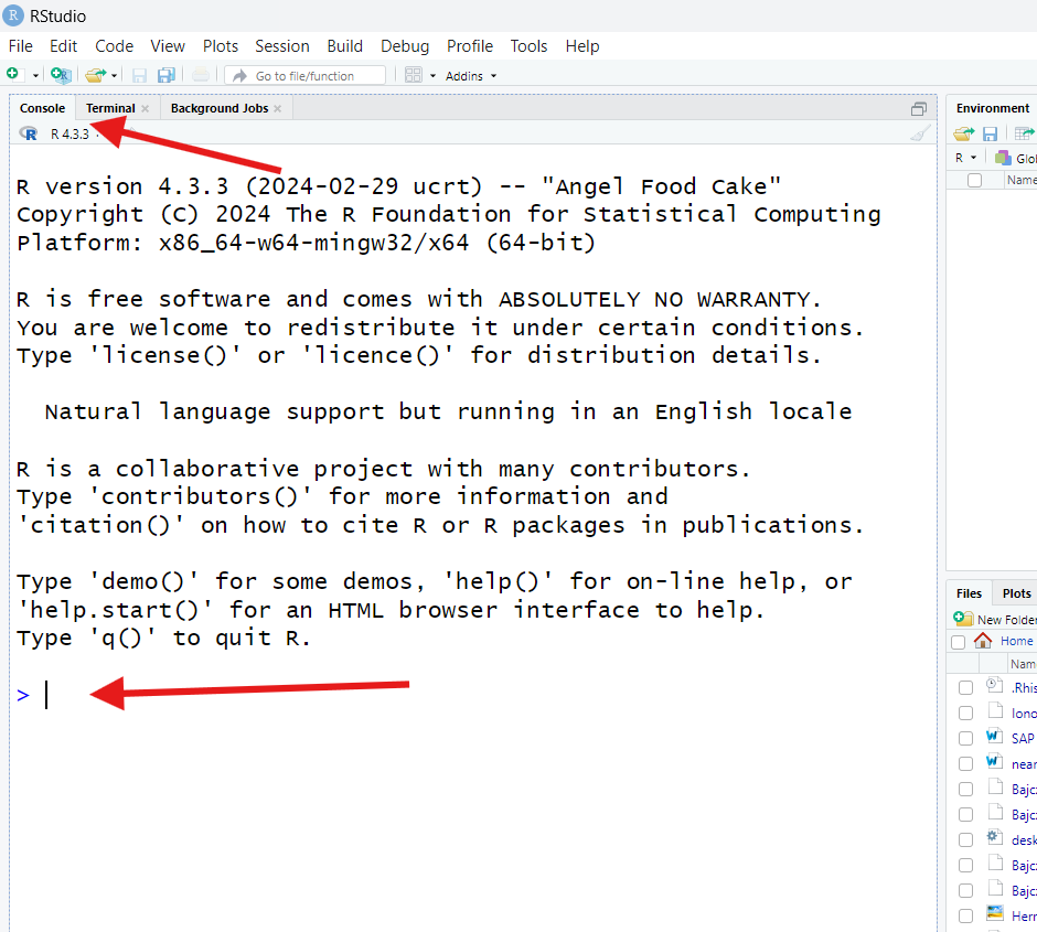
You’ll know you’ve found it if you see a > symbol at
the bottom and, when you click near that symbol, a
cursor (a blinking vertical line) appears next to
it.
Click near the > to receive the cursor. Then, type
exactly this:
R
2 + 3
Then, press your enter/return key. What happens?
You should receive something looking like this:
OUTPUT
[1] 5Since we know that two plys three is five, we can infer that R took
the values 2 and 3 and added them, given that
R sent 5 back to us. That must mean that + is
the symbol (programmers would call it an operator) R
uses as a shorthand for the verb “add.”
We’ve written our first R “sentence!” In programming, a complete, functional sentence is called a command because, generally, it is us commanding the computer to do something—here, add two values.
Challenge
Next, type exactly 2+3 into the Console and hit
enter/return. Then, type exactly 2+ 3 and hit enter/return.
What does R produce for us in each case? What does this tell us?
R doesn’t produce anything new, hopefully! We should get
5 back both times:
R
2+3
OUTPUT
[1] 5R
2+ 3
OUTPUT
[1] 5This teaches us our first R grammar (non-)rule—spaces don’t (usually) matter in R. Whether we put spaces in between elements of our command or not, R will read and act on (execute) them the same.
However, spaces do help humans read commands. Since you are a human (we assume!), it will probably help you read commands more easily to use spaces, so that’s what we’ll do with all the code in these lessons. Just know you don’t need them because they don’t convey meaning.
Math: The universal language
Next, type and run the following three commands at the Console (hit enter/return between each):
R
2 - 3
2 * 3
2 / 3
What does R produce for you? What does this tell us?
Here’s what you should have observed:
OUTPUT
[1] -1OUTPUT
[1] 6OUTPUT
[1] 0.6666667What that must mean is that -, *, and
/ are the R operators for subtraction,
multiplication, and division, respectively.
If nothing else, R is an extraordinary (if overpowered and over-complicated) calculator, capable of doing pretty much any math you might need! If you wanted, you could use it just for doing math.
Challenge
Next, try running exactly (2 + 3) * 5. Then, try running
exactly 2^2 + 3. What does R produce in each case, and
why?
In the first case, you’ll get 25 (and not 17, as you
might have expected). That’s because parentheses are R’s
operators for “order of operations.” Remember
those from grade school?? Things inside parentheses will happen
before things outside parentheses during math
operations.
So, 2 and 3 are added before any
multiplication occurs (try removing the parentheses and re-running the
command to confirm this).
In the second case, you’ll get back 7, as though
2^2 is really 4 somehow. This is because the
caret operator ^ is used for exponents in R. So,
2 gets raised to the power of 2
before any addition occurs, just as order of operations dictate
that it should.
These examples show that you can do any kind of math in R that you learned in school!
So far, we’ve seen what R will do for us if we give it complete commands. What happens if our command is incomplete?
At the Console, run exactly this:
What does R produce for you (or what changes)?
Your Console should now look something like this:
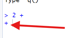
R has replaced the ready prompt > we
normally see in the Console with a + instead. This is R’s
waiting prompt, i.e., it’s waiting for us to
finish our previous command.
If we typed 3 and hit enter/return, we’d finish our
command, and we’d observe R return 5 and then switch back
to its ready prompt. If, however, we instead put in
another complete command, or another incomplete command that doesn’t
quite complete the previous command, R will remain confused and continue
giving us its waiting prompt. It’s easy to get “stuck” this way!
Callout
If you ever can’t figure out how to finish your command and get “stuck” on R’s waiting prompt, hit the “Esc” key on your keyboard while your cursor is active in the Console. This will clear the current command and restore the ready prompt.
No need to console me
By now, you might have realized that the Console is like a “chat window” we can use to talk to R, and R is the “chatbot” on the other side, sending us “answers” to our “questions” as quick as it can.
If we wanted, we could interact with R entirely through the Console (and, in fact, “base R” is more or less just a Console!).
However, we probably shouldn’t. Why not? For one thing, the Console is an impermanent record of our “chats.” If we close R, the contents of the Console get deleted. If we’d done important work, that work would be lost! Plus, the Console actually has a line limit—if we reach it, older lines get deleted to make room.
Sure, we could copy-paste the Consoles’ contents into another document on a regular basis, but that’d be a pain, and we might forget to do it sometimes. Not good!
In programming, the goal is to never lose important work! The Console just isn’t designed to prevent work loss. Thankfully, we have a better option…
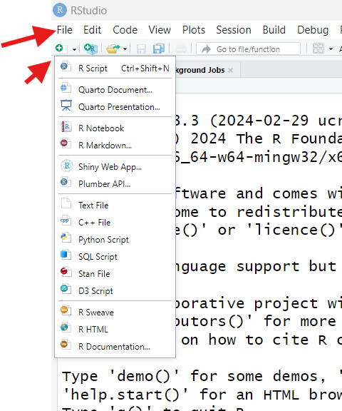
Staying on-script
Let’s open something called a script file (or “script” for short). Go to “File” at the top of your RStudio window, select “New File,” then select “R Script File.” Alternatively, you can click the button in the top-left corner of the RStudio window that looks like a piece of paper with a green plus sign, then select “R Script.”
Either way, you should now see a screen like this:
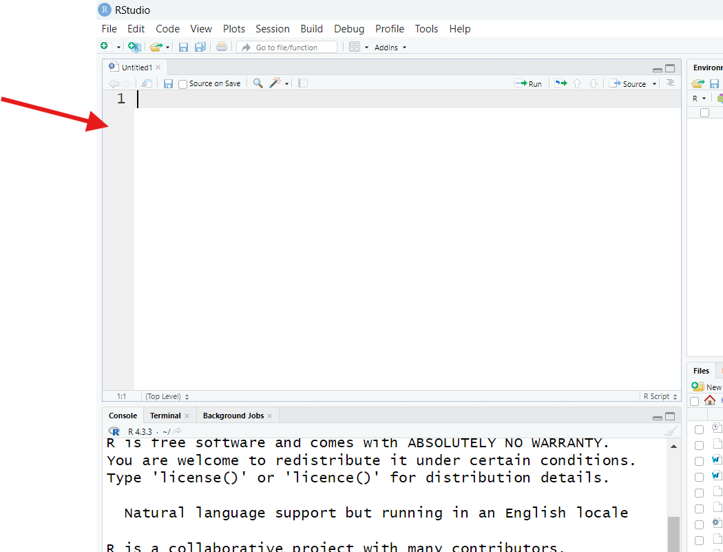
RStudio is displaying a blank script file. If you’re new to programming, a “script file” might sound scary, but a script file is just a text file, like one created in Microsoft Word or Google Docs, but even more basic—you can’t even format the text of one in any meaningful way (such as making it bold or changing its size).
Specifically, a script is a text file in which we write commands we are considering giving to R, like we’re writing them down in a notepad while we figure things out. Script files let us keep a permanent record of the code we’re crafting, plus whatever else we’re thinking about, so we can reference those notes later.
You might be wondering: “Why can’t I just have a Word file open with my code in it, then? Why bother with a special, basic text file?” The answer: In RStudio, script files get “plugged into” R’s Console, allowing us to pass commands from our script directly to the Console without copy-pasting.
Let’s see it! In your script file, type the following, then hit enter/return on your keyboard:
R
2 + 3
What happens in the Console?
The answer, you’ll discover, is nothing! Nothing new print to the Console. In our script, meanwhile, our cursor will move to a new line, just like in would in a word processor. This shows us that the “enter” key doesn’t trigger code to run in a script file, like it would at the Console.
Put your cursor back on the same line as 2 + 3 in your
script by clicking anywhere on that line, then find the button that says
“Run” in the upper-right corner of your Script pane (it looks like a
piece of paper with a green arrow through it pointing right).
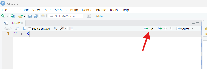
Once you find that button, press it.
What happens? This time, we observe our command and R’s response appear in the Console, as though we’d typed and ran the command there (but we didn’t!).
When we hit the “Run” button, R copied our command from our script file to the Console for us, then executed it.
This is the magic of script files:
- They serve as a permanent record of our code.
- They give us a place to “tinker” because we can decide if and when we run any code we put in one. Half the code in a script could be “experimental junk” and that’s ok, so long as you don’t personally find that confusing.
- You can run whichever commands from your script file whenever you want to, no copy-pasting necessary.
- When your commands get longer (wait until you see how long some
ggplot2commands get!), it’s easier to write them out and then format them to be human readable in a script file than it would be at the Console.
So, few everyday R users code exclusively at the Console these days. Instead, they code in scripts, letting R “teleport” relevant commands to the Console when they’re ready. As such, we encourage you to code entirely from a script for the rest of these lessons.
Leaving a legacy
You may have noticed that, when you first typed something in your script file, its name (found in the tab above it), turned red and got an asterisk placed next to it:
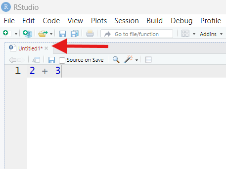
This means our script has unsaved changes. To fix that, go to “File”, then select “Save.” Or, you can hit Control+S on your keyboard, or press the blue “disk” button in the top-left corner of the Script pane (just below the arrowhead in the picture above).
If your script already has a name, doing any of these will save the file. If it doesn’t have a name, you’ll be prompted to give it one as you save it. [R scripts get the file extension “.R” to indicate that they are “special.”]
Callout
One of programming’s cardinal rules is “save often!” Your script file is only a permanent record of your work if you remember to save your work regularly!
Challenge
Scripts may permanently save your code, but not everything in a script needs to be code!
Type and run the following from a script : #2 + 5.
What happens in the Console? What does this teach us?
In this case, R will print your command in the Console, but it won’t
produce any output. That is because # is
R’s comment operator. A comment is anything that
follows a # in the same coding “line.” When R encounters
a comment while executing code, it skips it.
This means that you can leave yourself notes that R will ignore, even if they are interspersed between functional commands!
Callout
Writing comments explaining your code (what it’s for, how it works, what it requires, etc.) is called annotating. Annotating code is a really good idea! It helps you (and others) understand your code, which is particularly valuable when you’re still learning. As we proceed through these lessons, we highly recommend you leave yourself as many helpful comments as you can—it’ll make your script a learning resource in addition to a permanent record!
(Section #2) Objects of our affection
At this point, we know several fundamental R concepts:
Spaces don’t (generally) matter (except that they make code easier for us humans to read).
Line breaks (made with the enter key) do matter (if they make a command incomplete).
Commands can be complete or incomplete, just like sentences can be complete or incomplete. If we try to execute an incomplete command, R expects us to finish it before it’ll move on.
R has a number of symbols (operators) with particular meanings, such as
#and*.R will ignore comments (anything on a line following a
#), and annotating our code with comments is good.Writing code in scripts is also good.
We’ve taken our first steps towards R fluency! But, just as it would be for a human language, the next step is a big one: We need to start learning R’s nouns.
Assignment and our environment
In your script, run 5 [Note: besides hitting the “Run”
button, you can press control/command+enter on your keyboard to run
commands from a script].
R
5
OUTPUT
[1] 5R just repeats 5 back. Why? Because we didn’t tell R to
do anything with 5; it could only assume we wanted
5 returned as a result.
Important: This is, in a nutshell, how our
relationship with R works—it assumes we are giving
commands (“orders”) for which we’ll provide
inputs R should use to carry out those “orders” (in
this case, our input was 5). R will then execute
those commands by doing some work and returning some
outputs (in this case, the output was also
5).
In broad strokes, any single input we give R, or any single output we receive from R, is a “noun” in the R language—these nouns are called objects (or, sometimes, variables).
The 5s we’ve just seen are “temporary,” or
unnamed, objects. They exist only as long as it takes R to work
with or yield them, after which R promptly forgets they exist (it’s like
R has extreme short-term memory loss!).
However, if we don’t want R to forget a noun, we can prevent it. In your script, run the following:
R
x = 5
What happens in the Console when this command runs? Do you notice anything different or new in your RStudio window?
At first, it might seem like nothing’s happened; R reports our command in the Console but no outputs, just like when we ran a comment.
However, find the pane labeled “Environment” (it’s most likely in the upper-right, though it could be somewhere else). Once you’ve found it, if it says “Grid” in the top-right corner, good! If it says “List” instead, click that button and switch it to “Grid.”
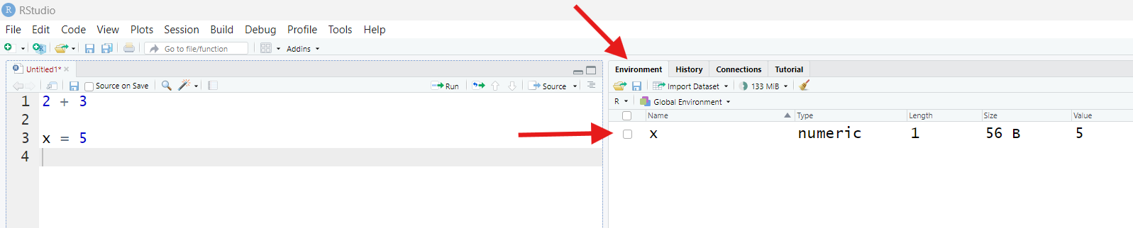
Before now, this pane may have said “Environment is empty.” Now, it
should instead list something with the Name x, a Value of
5, a Length of 1, and a Type of
numeric.
What’s happened? Let’s experiment! In your script, run:
R
x + 4
R will return:
OUTPUT
[1] 9This is interesting. In English, adding 4 to a letter is
non-sensical. However, R not only does it (under these circumstances,
anyway!), but we get a specific answer back. It’s as if R now knows,
when it sees x, that what it should think
is 5.
That’s because that’s exactly what’s happening! Earlier, with our
x = 5 command, we effectively taught R a new “word,”
x, by assigning a value of 5
to a new object by that name (= is R’s
assignment operator). Now, whenever R sees
x, it will swap it out for 5 before doing any
operations.
x is called a named object. When we
create named objects, they go into our Global
Environment (or “environment” for short). To understand what
our environment is, imagine that, when you start up R, it puts
you inside a completely empty room.
As we create or load objects and assign them names, R will start filling this room with bins and shelves and crates full of stuff, each labeled with the names we gave those things when we had R create them. R can then use those labels to find the stuff we’re referencing when we use those names.
At any time, we can view this “room” and all the named objects in it: That’s what the Environment pane does.
Once we have named an object, that object will exist in our Environment and will be recognized by R as a “word” until we either:
Remove it, which we could do using the
rm()function (more on functions later) or by using the “clear objects” button in the Environment pane (it looks like a broom).We close R (R erases our environment every time we exit, by default).
The fact that our entire environment is lost every time we close R may sound undesirable (and, when you’re learning, it often is!), but the alternative would be that our “room” (environment) just gets more and more clogged with stuff. That’d create problems too!
Callout
Besides, the point of working in a script is that we can keep all the code we need to remake all our needed named objects, so we should never have to truly “start over from scratch!”
Besides looking at your environment, if you want to see the contents
of a named object (hereafter, we’ll just call these “objects”), you can
have R show you its contents by asking R to print that object.
You can do this using the print() function or simply by
executing only the object’s name as a command:
R
print(x)
OUTPUT
[1] 5R
x
OUTPUT
[1] 5Naming an object may not seem like much of a “feature” to you now
(it’s not like 5 is harder to type than x!),
but an entire 30,000 row data set could also be a single object
in R. Imagine typing that whole thing out every time you want to
reference it! So, being able to give an input/output, no matter its size
or complexity, a brief “nickname” is actually very handy.
Naming rules and conventions
Let’s talk about the process of naming objects (assignment) in more detail.
In your script, type the following, but don’t execute it just yet:
R
y = 8 + 5
Guess what R will do when you provide it with this command. Then, execute the command and see if you were right!
You should see y appear in your environment. What
“Value” does it have? Is that what you thought it would be?
R
y = 8 + 5
y
OUTPUT
[1] 13We get back a Value of 13 for y. What this
tells us is that, when R executed our command, it did so in a particular
way:
It first did the stuff we’ve asked it to do on the right-hand side of the
=operator (it added two numbers).Then it created an object called
yand stuffed it with the result of that operation. This is why ouryhas a value of13and not8 + 5.
This may seem strange, but, at least for assignment, R kind of reads right to left in that it assumes we want to store the result of operations inside objects, not the operations themselves. As we’ll see, this is not the only way that R reads a command differently than you or I might read text.
Time for our next experiment. Execute the following command:
R
y = 100
What happens, according to your Environment pane? Is that what you expected to happen?
If you look in your environment, there will still be one (and only
one) object named y, but it’s Value will have changed to
100. This demonstrates two things about how assignment
works in R:
Object names in R must be unique—you can have only one object by a specific name at a time.
If you try to create a new object using an existing object’s name, you will overwrite the first object with the second; the first will be permanently lost!
This is why it’s really important to pick good names for your objects—more on that in a second.
Next, type and run the following:
R
Y = 47
What does the Environment pane report now? Is that what you expected?
You should see an object called Y appear in your
environment. Meanwhile, y is also there, and it’s value
hasn’t changed. What gives—didn’t we just establish that names
had to be unique??
Well, they do! But R is a case-sensitive programming language.
This means that, to R, Y is different from y.
So, Y and y are completely different “words,”
as far as R is concerned!
Callout
For beginning programmers, forgetting about case sensitivity is the number-one source of errors and frustration! If you learn absolutely nothing else from these lessons, learn that you can’t be “casual” about upper- versus lowercase letters when you are coding!
Let’s continue experimenting. Run the following two commands:
What happens? What does this experiment teach us?
The first command runs fine—we get a new object named z1
in our environment. This teaches us that including numbers in object
names in R is ok.
I am error
However, the second command does not result in a new object
called 1z. Instead, R returns an error
message in the Console. Uh oh! Error messages are R’s way of saying
that we’ve formed an invalid command.
To be completely frank, R’s error messages are generally
profoundly unhelpful when you’re still learning. This one, for
example, says Error: unexpected symbol in "1z" . What the
heck does that even mean?!
Well, to translate, it’s R’s way of saying that while numbers
are allowed in object names, your object names can’t
start with numbers. So, the 1 at the beginning
is an “unexpected symbol.”
When you get error messages in R, you might get frustrated because you will know you did something wrong but you may not be able to figure out what that something was. Just know this will improve with time and experience.
Callout
In the meantime, though, here are two things you should always try when you get an error message and don’t immediately know what your mistake was:
Check for typos. 95% of error messages are R’s cryptic way of saying “I’m not 100% sure that I know which object(s) you’re referring to.” For example, as we saw earlier,
variable1would be a different word thanVariable1or evenvarible1, so start troubleshooting by making sure you didn’t mix up capital and lowercase letters or add or remove characters.Try Googling the exact error message. It’s likely one of the first results will have an explanation of what may cause that particular error. (An even better option these days might be asking a derivative AI program like ChatGPT to explain the error to you, if you also provide the code that caused it!)
Errors are an inevitable consequence of coding. Don’t fear them; try to learn from them!
As you use R, you will also encounter warnings. Warnings are also messages that R prints in the Console when you run certain commands. It’s important to stress, though, that warnings are not errors. An error means R knew it couldn’t perform the operation you asked for, so it gave up; a warning means R did perform an operation, but it’s unsure if it did the right one, and it wants you to check.
A quick way to see a warning is to try “illogical math,” like logging a negative number:
R
log(-1)
WARNING
Warning in log(-1): NaNs producedOUTPUT
[1] NaNHere, R did something, but it might not have been the
something we wanted [NaN is a special value
meaning “not a number,” which is R’s way of saying “the math you just
had me do doesn’t really make sense!”].
The line between commands so invalid that they produce errors and commands just not invalid enough to produce warnings is thin, so you’re likely to encounter both fairly often.
Going back to our “room”
Anyhow, let’s return to objects: Try the following commands:
What happens? What does this teach us?
The first command runs fine; we see object_1 appear in
our environment. This tells us that some symbols are allowed in
R object names. Specifically, the two allowable symbols are
underscores _ and periods ..
The second command returns an error, though. This tells us that spaces are not allowed in R object names.
Here’s one last experiment—Type out the following commands, consider what each one will do, then execute them:
R
x = 10
y = 2
z = x * y
y = -1000
z
OUTPUT
[1] 20What is z’s Value once these commands have run? What did
you expect its Value to be? What does this teach us?
Here, we created an object called z in the third command
by using two other objects, x and y in the
assignment command. We then overwrote the previous
y’s Value with a new one of -1000. However,
z still equals 20, which is what it was before
we overwrote y.
This example shows us that, in R, making objects using other
objects doesn’t “link” those objects. Just because
we made z using y doesn’t mean z
and y are now “linked” and z will
automatically change when y does. If we change
y and want z to change too, we have to
re-run any commands used to create z.
This is actually a super important R programming concept: R’s objects never change unless you run a command that explicitly changes them. If you want an R object to “update,” a command must trigger that!
It’s natural to think as though computers will know what we want and automate certain tasks, like updating objects, for us, but R is actually quite “lazy.” It only does exactly what you tell it to do and nothing more, and this is one very good example.
What’s in a name?
We’ve learned how we can/can’t name objects in R. That brings us to how we should/shouldn’t name them.
In programming, it’s good practice to adopt a naming convention. Whenever we name objects, we should do it using a system we use every single time.
Why? Well, among other reasons, it:
Prevents mistakes—you’ll be less likely to mess up or forget names.
Saves time because coming up with new names will be easier and remembering old names will be faster because they’re predictable.
Makes your code more readable, digestible, and shareable.
Our goal should be to create object names that are unique, descriptive, and not easily confused with one another but, at the same time, aren’t a chore to type or inconsistent with respect to symbols, numbers, letter cases.
So, by this logic, y is a terrible name! It
doesn’t tell us anything about what this object stores, so we’re
very likely to accidentally overwrite it or confuse it with
other objects.
However, rainfall_Amounts_in_centimetersPerYear.2018x is
also a terrible name. Sure, it’s descriptive and unique, and we
wouldn’t easily mix it up with others object, but it’d be a pain to
type! And with the inconsistencies in symbol and capital letter usage,
we’d typo it a lot.
Here are some example rules from a naming convention, so you can see what a better way to do things might look like:
All names consist of 2-3 human “words” (or abbreviations).
All are either in all caps
LIKETHISor all lowercaselikethis, or if capitals are used, they’re only used in specific, predictable circumstances (such as proper nouns).-
Words are separated to make them more readable.
- Some common ways to do this include using so-called snake_case, where words are separated by underscores, dot.case, which is the same using periods, or camelCase, where one capital is used after where a space would have been.
Numbers are used only when they convey meaning (such as to indicate a year), not to “serially number” objects like
data1,data2,data3, etc. (such names are too easy to confuse and aren’t descriptive).Only well-known abbreviations are used, such as
wgtfor “weight.”
Making mistakes in any language is frustrating, but they can be more frustrating when you’re learning a programming language! It may seem like a hassle, but using a naming convention will prevent a lot of frustrating mistakes.
Discussion
Pause and jot down several rules for your own personal naming convention.
There are no “right answers” here. Instead, I’ll give you a couple of rules from my own personal naming convention.
First, generally speaking, column names in data sets are written in ALLCAPS. If I need to separate words, I do so using underscores. My comments are also written in ALL CAPS to make them stand out from the rest of my code.
Meanwhile, I only use numbers at the ends of names, and I never use periods.
Lastly, I use snake_case for function names (more on functions in a bit), but I use camelCase for object names.
One last thing about assignment: R actually has a
second assignment operator, the arrow
<-. If you use the arrow instead of = in an
assignment command, you’ll get the same result! In fact,
<- is the original assignment operator;
= was added recently to make R a bit more like other common
programming languages.
In help documents and tutorials, you will often see
<- because it’s what a lot of long-time R users are used
to. Also, = is used for not one but several other
purposes in R (as we’ll see!), so some beginners find it confusing to
use = for assignment also.
Throughout, these lessons use = for assignment because
it’s faster to type (and what the instructors are used to). However, if
you would prefer to use <-, go for it! Just recognize
that both are out there, and you are likely to encounter both as you
consume more R content.
Just typical
Earlier, when we made x and assigned it a value of
5, R reported its Type as numeric in our
environment. What does “Type” mean?
Computers, when they store objects in their “heads,” have particular ways of doing so, usually based on how detailed the info being stored is and how this info could later be used.
Numeric data (numbers with potential decimals) are quite detailed, and they can be used in math operation. As such, R stores these data in a specific way acknowledging these two facts.
Let’s see some other ways R might store data. In your script, run the following commands, paying close attention to punctuation and capitalization:
R
wordString = "I'm words" #Note the use of camelCase for these object names :)
logicalVal = FALSE
You should get two new objects in your environment. The first should
have a Type of character. This is how R stores text
data.
Discussion
Note we had to wrap our text data in quotes
operators " " in the command above.
Text data must always be quoted in R. Why? What would
happen if we tried to run x = data instead of
x = "data", for example?
As we have seen, R thinks unquoted text represents a potential object name. So, to make it clear that we are writing textual data and not an object name, we quote the text.
In our hypothetical example, if we tried to run
x = "data", we’d store the value of "data" in
an object called x. If, instead, we ran
x = data, R would look for an object called
data to work with instead. If such an object exists, its
current value inside a second object called x. But, if no
such object existed, R would instead return an error, saying it couldn’t
find an object named data.
Forgetting to quote text is an extremely common mistake when learning R, so pay close attention to the contexts in which quotes are used in these lessons!
Text data can also be detailed (a whole book could be a single text object!) but they can’t be used for math, so it makes sense R uses a different Type to store such data.
The second object above (logicalVal) has a Type of
logical. Logical data are “Yes/No” data. Instead of storing
these data as “Yes” or “No,” though, a computer stores them as
TRUE or FALSE (or, behind the scenes, as
1 or 0). These data are not detailed compared
to others we’ve seen, so it makes sense there’s another type for storing
them. We’ll see what logical data are for in a later section.
You can think of types as R’s “adjectives:” They describe what kinds of objects we’re working with and what can and can’t be done with them.
There are several more object Types we’ll meet, but before we can, we need to take our next big step: we need to learn about R’s verbs.
(Section #3) Function junction
Earlier, we established that our relationship with R is one in which we provide R with inputs (objects) and commands (“orders”) and it responds by doing things (operations) and producing outputs (more objects). But how does R “do things?”
Just as with a human language, when we’re talking actions, we’re talking verbs. R’s verbs are called functions. Functions are bundles of one (or more) pre-programmed commands R will perform using whatever inputs it’s given.
We’ve actually met an (unusual) R function already: +.
This symbol tells R to add two values (those on either side of it). So,
a command like 2 + 2 is really a bundling together of our
inputs (2 and 2) and an R verb (“add”).
Most R verbs look different from +, though. In your
script, run the following:
R
sum(2, 5)
What did R do? What does this teach us?
We’ve just successfully used sum(), R’s more
conventional, general verb for “add the provided stuff,” and it is a
good example of how functions work in R:
Every function has a name that goes first when we’re trying to use that function.
Then, we add to the name a set of parentheses
( ). [Yes, this is a second, different use of parentheses in R!]Then, any inputs we want that function to use get put inside the parentheses. Here, the inputs were
2and5. Because we wanted to provide two inputs and not just one, we had to separate them into distinct “slots” using commas,.
If we omit or mess up any of those three parts, we might get an unexpected result or even an error! Just like any language, R has firm rules, and if we don’t follow them, we won’t get the outcome we want.
Side-note: In programming, using a function is referred to as
calling it, like it’s a friend you’re calling up on the phone
to ask for a favor. So, the command sum(2, 5) is a
call to the sum() function.
Challenge
As we’ve seen, R is a powerful calculator. As such, it has many math
functions, such as exp(), sqrt(),
abs(), sin(), and round(). Try
each and see what they do!
exp() raises the constant e to the power of
the provided number:
R
exp(3)
OUTPUT
[1] 20.08554sqrt() takes the square root of the provided number:
R
sqrt(65)
OUTPUT
[1] 8.062258abs() determines the absolute value of the provided
number:
R
abs(-64)
OUTPUT
[1] 64sin() calculates the sine of the provided number:
R
sin(80)
OUTPUT
[1] -0.9938887round() rounds the provided number to the nearest whole
number:
R
round(4.24)
OUTPUT
[1] 4Pro-to types
R also has several functions for making objects, including some important object types we haven’t met yet! Run the following command:
R
justANumber = as.integer(42.4)
This command produces an object of Type integer. The
integer type is for numbers that can’t/don’t have decimals, so any data
after the decimal point in the value we provided gets lost, making this
new object’s Value 42, not 42.4.
Next, run:
R
numberSet = c(3, 4, 5)
This produces an object containing three Values (3,
4, and 5) and is of Type numeric,
so it maybe doesn’t look all that special at first.
The product of a c() function call is special
though—this function combine (or
concatenates) individual values into a unified
thing called a vector. A vector is a set of values
grouped together into one object. We can confirm R thinks
numberSet is a vector by running the following:
R
is.vector(numberSet)
OUTPUT
[1] TRUETo which R responds TRUE (which means “Yes”).
If a single value (also called a scalar) is a single point in space (it has “zero dimensions”), then a vector is a line (it has “one dimension)”. In that way, our vector is different from every other object we’ve made until now! That’s important because most R users engage with vectors all the time—they’re one of R’s most-used object types. For example, a single row or column in data set is a vector.
One reason that vectors matter is that many functions in R are vectorized, meaning they operate on every entry inside a vector separately by default
To see what I mean, run the following:
R
numberSet - 3
OUTPUT
[1] 0 1 2What did we receive? What did this teach us?
R returns a vector of the same length as numberSet but
containing 0, 1, and 2, which are
what you’d get if you had subtracted 3 from each entry in
numberSet separately. That’s vectorization! More on that in
a later lesson.
So, most R functions are designed to work not just on lone values but
on vectors, and some even expect their inputs to be vectors. A
good example is mean(), which takes the average of the
provided inputs. Yes, you could take the average of just one
value, but it’d be pretty pointless! So it makes sense this function
expects a vector and not a scalar as an input.
Let’s try it. Run:
R
mean(numberSet)
OUTPUT
[1] 4Vectors can hold non-numeric data too. For example, (carefully) type and run the following:
R
charSet = c("A", "B", "B", "C")
This will create a character vector. If we check our
environment, we will notice it has a Length of 4, due to
its four entries. If you ever want to see the length of a vector, you
can use the length function:
R
length(charSet)
OUTPUT
[1] 4Timeout for factors
We can use charSet to discover another, special R object
Type. Run:
R
factorSet = as.factor(charSet)
If you check your environment after this command, you’ll see we’ve
made an object of Type factor. What’s a factor??
Factors are a special way R can store categorical data (data that belong to different, discrete categories that cannot be represented meaningfully with numbers, such as “male”, “female”, and “neuter”).
To create a factor, R:
Finds all the unique categories (here, that’s
A,B, andC).Picks a “first” category. By default, it does this alphanumerically, so
Ais “first.”It turns each category, starting with the first, into a “level,” and it swaps that category out for an integer starting at
1. So,Abecomes level1,Bbecomes level2, and so on.
This means that, under the hood, R is actually now storing these text data as numbers and not as text. However, it also stores which categories goes with which numbers. That way, at any time, it can “translate” between the numbers it’s storing and the text values in the original data. So, whenever it makes sense to treat these data as text, R can do that, and whenever it’d be easier for them to be “numbers” (such as when making a graph), R can do that too!
We can see all this underlying structure using the structure
function, str():
R
str(factorSet)
OUTPUT
Factor w/ 3 levels "A","B","C": 1 2 2 3This will show that R now thinks of our A, B, B, C data
as 1, 2, 2, 3, but it hasn’t forgotten that 2
really means B.
For certain operations, factors are very convenient. Part of why R became so beloved by statisticians was because of factors!
However, if you think factors are weird, you’re right—they are. If you don’t want to use them, increasingly, you don’t have to; they are sort of falling out of favor these days, truth be told. But they are still common enough that it pays to be aware of them.
2D or not 2D
Moving on, we have another two important objects to meet: Matrices and data frames. Type (carefully) and run the following:
R
smallMatrix = matrix(c(1, 2, "3", "4"))
This command demonstrates another fundamental concept: In R, you can stuff functions calls inside other function calls. This is called nesting.
When we nest, R reads our command from the “inside out,”
evaluating inner operations first before tackling outer ones. So, here,
R first creates a vector containing the values 1,
2, "3", and "4". It then
provides that vector to the matrix() function, which
expects to be given a vector of values it can arrange into a matrix
format.
As such, we don’t have to stop and name every object we want to use—we can choose to use or create unnamed objects if that’s our preference.
However, for many beginners, reading nested code can be tricky, and not saving “intermediate objects” feels wrong! If you’d prefer, you can always write commands one at a time rather than nest them; it’ll take more time and space, but you might find it more readable. For example, here, you could have instead done something like this:
R
smallMatrixVec = c(1, 2, "3", "4")
smallMatrix = matrix(smallMatrixVec)
Anyhow, we can see our matrix by running just its name as a command. When we do that, we see this:
R
smallMatrix
OUTPUT
     [,1]
[1,] "1"
[2,] "2"
[3,] "3"
[4,] "4"
If a vector is a one-dimensional set of values, then a matrix is a
two-dimensional set of values, arranged in rows and columns. Here,
we created a matrix with one column (marked at the top with
[,1]) and four rows (marked along the left side with
[1,], [2,], and so on).
Discussion
Notice that all values in our matrix are now text (they are
surrounded by "s), even the 1 and
2 we originally entered as numbers. Why do you think this
happens?
Vectors and matrices (most objects, really!) in R can only hold values of a single Type. If we try to put multiple value types into one object, R will change (or coerce) the more complex/versatile type(s) into the simpler/less versatile type(s). In this case, it turned our numeric data (which can be used for math) into character data (which can’t be used for math).
Why does R coerce dara? Well, remember—many operations in R are
vectorized, meaning they happen to all values in an
object simultaneously and separately. This means we could run a command
like smallMatrix + 4 to try to add 4 to
all values in our matrix. This would make sense for our numbers
but not for our text!
Rather than giving us the opportunity to make mistakes like that, R “reduces” all values in an object to the “simplest” available type so that we never try to do “more” with an object’s values than we should be able to.
So data coercion makes sense, when you think about it. However, what if you have a data set that contains both text and numeric data? R has you covered, so long as those data are in different columns! Run the following:
R
smallDF = data.frame(c(1,2), c("3", "4"))
Follow this with smallDF as a command to see the
result:
R
smallDF
OUTPUT
  c.1..2. c..3....4..
1       1           3
2       2           4
This time, we get an object of Type data.frame. Data
frames are another special R object type! Like a matrix, a data frame
is a 2D arrangement of values, with rows and columns (albeit marked
differently than those in our matrix).
However, this time, when we look at our new data frame in the Console, it looks like R has done the opposite—it looks like it has turned our text into numbers!
But, actually, it hasn’t. To prove it, we can use the structure
function, str(), to look under the hood at
smallDF. Type and run the following:
R
str(smallDF)
OUTPUT
'data.frame':	2 obs. of  2 variables:
 $ c.1..2.    : num  1 2
 $ c..3....4..: chr  "3" "4"
You should get output like this:
OUTPUT
'data.frame':	2 obs. of  2 variables:
 $ c.1..2.    : num  1 2
 $ c..3....4..: chr  "3" "4"
On the left-hand side of the output is a list of all the columns in our data frame and their names (they’re weird here because of how we made our data frame!).
On the right-hand side is a list of the Types of each column and the
first few values in each one. Here, we see that, actually, the second is
still of Type character (“chr” for short). The quotes
operators just don’t print when we look at a data frame.
The str() output shows that we have, in the same object,
two columns with different data types. It’s this property that makes
data frames special, and it’s why most R users engage with data frames
all the time—they are the default object type for storing data sets.
Note that every column can still only contain a single data type, so you can’t mix text and numbers in the same column without coercion happening.
Another object type R users encounter often is lists. Lists are useful but also weird; we’re not going to cover them here, but, if you’re curious, you can check out this resource to become better acquainted with them. There are also objects that can hold data in 3 (or more) dimensions, called arrays, but we won’t cover them here either because most users won’t need to use them much, if ever.
For argument’s sake
Earlier, we saw that functions get inputs inside their parentheses
( ) and, if we are giving a function multiple inputs, we
separate them using commas ,. This helps R know when one
input ends and another begins.
You can think of these commas as creating “slots,” with each slot receiving one input. These “slots” may feel like things we, the users, create as we call functions, but they actually aren’t!
When a programmer creates a function, they need to ensure that the user knows what inputs they are expected to provide (so we’re not providing illogical types of inputs or an inadequate number of them). Meanwhile, R needs to know what it’s supposed to do with those inputs, so it needs to be able to keep them straight.
The programmer solves these two programs by designing each function to have a certain number of input slots (these are called parameters). Each slot is meant to receive an input (formally called an argument) of a particular type, and each slot has its own name so R knows which slot is which.
…This’ll make much more sense with an example! Let’s consider
round() again. Run the following:
R
round(4.243)
OUTPUT
[1] 4We get back 4, which tells us that round()
rounds our input to the nearest whole number by default. But what if we
didn’t want to round quite so much? Could we round to the nearest tenth
instead?
Well, round(), like most R functions, has more than one
input slot (parameter); we can give it not only numbers for it
to round but instructions on how to do that.
round()’s first parameter (named x) is the
slot for the number(s) to be rounded—that’s the slot we’ve already been
providing inputs to. Its second parameter slot (named
digits), meanwhile, can receive a number of decimal places
to round those other inputs to.
By default, digits is set to 0
(i.e., don’t round to any decimal place; just give back whole
numbers). However, we can change that default if we want. Run the
following:
R
round(4.243, 1)
OUTPUT
[1] 4.2By placing a 1 in that second input slot, we’ve asked R
to round our first input to the nearest tenth instead.
Challenge
We can learn more about how functions work with some experiments. Type the following into your script, but don’t run it yet:
R
round(1, 4.243)
This is the exact same inputs we gave round() before,
just reversed. Do you think R will generate the same output? Why or why
not? Try it and observe what you get.
R
round(1, 4.243)
OUTPUT
[1] 1You get back 1, which is not the same answer as we got
before. Why?
We essentially just asked R to round 1 to
4.243 decimal places. Since that doesn’t really make sense,
R assumes we meant “round to 4 decimal places.” However, since
1 is already fully rounded, there’s no need to round it
further.
The experiment in the exercise above shows that, for R functions, input order matters. That is, specific slots are in specific places inside a function’s parentheses, and you can’t just put inputs into slots all willy-nilly!
…Or maybe you can, if you’re a little more thoughtful about it. Try this instead:
R
round(digits = 1, x = 4.243)
This time, you should get back 4.2, like we did the
first time.
OUTPUT
[1] 4.2This is because we have used the parameter names (to the left of the
=s) to match up our inputs (to the right of the
=s) with the specific slots we want them to go into. Even
though we provided the inputs in the “wrong” order, as far as how
round() was programmed, we gave R enough information that
it could reorder our inputs for us before doing continuing.
When in doubt, always “name” your arguments (inputs) in this way, and you’ll never have to worry about specifying them in the wrong order!
Note—we’ve just seen a second use for the = operator.
Until now, we’ve only used = to create new named
objects (assignment). Here, we’re matching up
inputs with input slots (we’re naming our
arguments). In both cases, names are involved, but, in
the latter, nothing new is actually being created or added to R’s
vocabulary.
Challenge
I mentioned that some folks find it confusing that = has
multiple different uses. Let’s see if you might be one of those people.
Consider the following command:
R
newVar = round(x = 4.243, digits = 4)
Can you explain what this command does?
First off, we could have written this same command this way instead:
R
newVar <- round(x = 4.243, digits = 4)
We’re asking R to create a new named object called
newVar; that new object will contain the result of a
call to round(). This assignment task is
facilitated by the = operator (but could just as easily
have been facilitated by the <- operator).
For our round() call, we’ve provided two inputs, an
x (a value to round) and a number of digits to
round that value to. We’ve ensured R knows which input is which by
naming the slots we want each to go into. This input-slot matching is
facilitated by the = operator also (the <-
operator would NOT work for this purpose).
If it feels harder to read and understand commands that use the same
operator (=) for two different purposes, that’s ok! Just
switch to <- for assignment.
Notice that we can call round() with or without
giving it anything for its digits parameter. It’s
as though that slot is “optional.”
That’s because it is! Some input slots have default values their designers gave them. If we’re ok with those defaults, we don’t need to mess with their slots at all. Many optional inputs are there if you want to tweak how R performs a more basic operation. In that way, they are kind of like R’s adverbs, if you think about it!
By contrast, try this command:
R
round(digits = 1)
You’ll get an error. What is this error telling us?
The error will say
Error: argument "x" is missing, with no default. This is
actually a pretty informative error, for a change! We know, now, that
the number(s) we want to round go in a slot named x. In the
example above, we know we didn’t provide any inputs for x,
so our x input is indeed “missing.”
It makes sense this would be a problem—understandably,
round() has no default for x. How could it?
Are we expecting R to somehow guess what value(s) we are hoping to
round, out of all possible values?? That would be an
insane expectation!
So, while some function inputs might be optional, others are required because they have no defaults. If you try to call a function without specifying all required inputs, you’ll usually get an error.
Next, let’s try this command:
R
round(x = "Yay!")
This will also trigger an error, with another error message you should hopefully be able to decode!
The error says
Error in round: non-numeric argument to mathematical function.
Basically, it’s saying “Hey! You just tried to get me to do math on
something that is clearly not a number!”
This shows that each input probably needs to be of a specific form or Type so that a function’s operations are more likely to work as planned.
Getting help
By this point, you might be wondering: “But how would I know what input slots a function has? Or what types or forms of inputs I should be providing? Or what what those slots are named? Or what order those slots are in? Or which slots are required?”
These are all super good questions! Thankfully, there’s an easy answer to them all—we can look them up! Run the following command:
R
?round #You can run this with or without ()s
This command should trigger your RStudio to show its Help pane, generally found in the bottom-right corner (though it could be somewhere else).
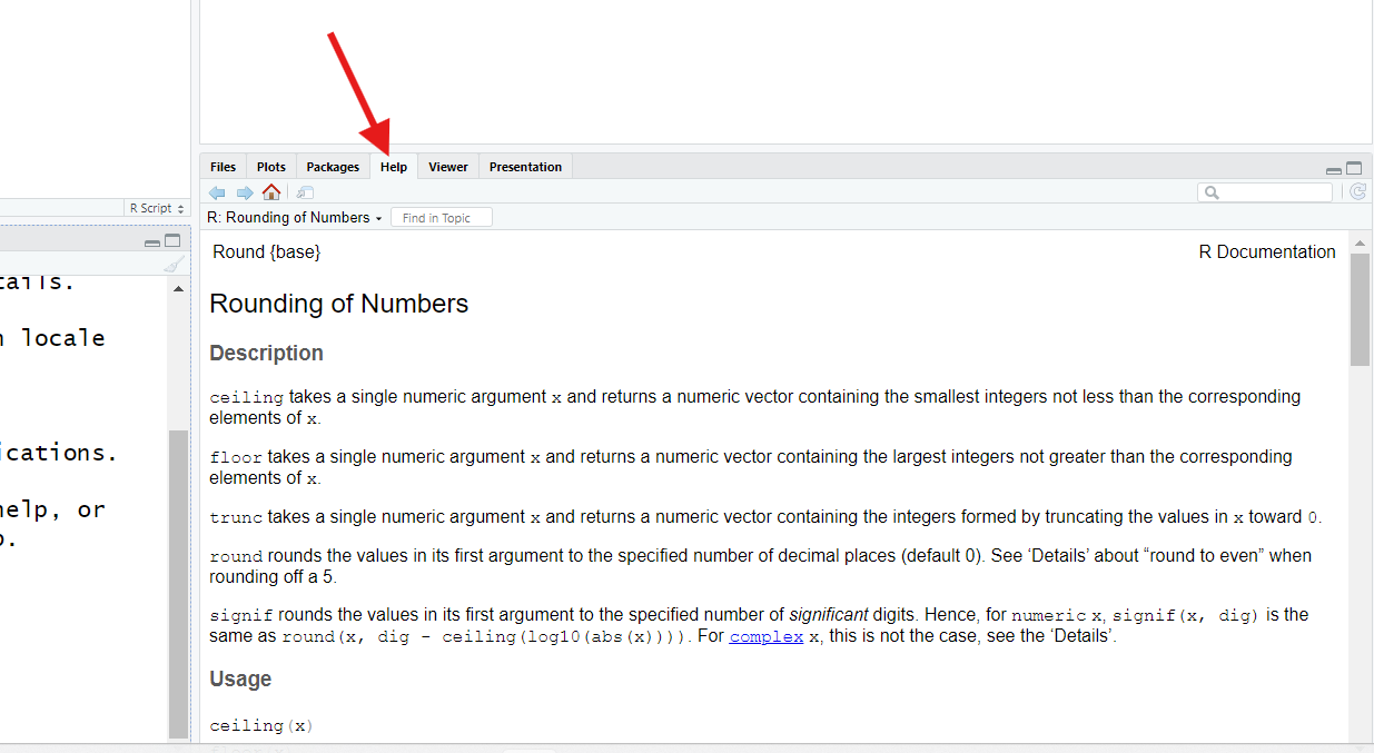
The ? operator, when used in front of a function’s name,
will bring up the help page for that function.
Fair warning: These are not always the easiest pages to read! In general, they are pages written by programmers for programmers, and it shows.
However, already, you might discover you understand more of this page’s contents than might think. Here’s what to look for when reading a function’s help page:
The function’s name is at the top, along with the name of the package it’s from in braces
{ }.roundis in thebasepackage, which means it comes with “base R.”The
Descriptionsection describes (hopefully clearly!) what the function’s purpose is, generally. If a number of related functions can logically share the same help page (as is the case here), those other functions will be listed and described here too.The
UsageandArgumentssections show the input slots for this function, their names, and the order they’re expected in. You should see, in theUsagesection, thatxanddigitsare the first and second inputs forround().In the
Argumentssection, you can read more about what each input slot is for (they are also listed in order). If there are any form or type requirements for an input, those will (hopefully) be noted here.The
Detailssection is one you can generally skip; it typically holds technical details and discusses quirky edge cases. But, if a function seems to be misbehaving, it’s possibleDetailswill explain why.At the bottom, the
Examplessection shows some code you could run to see a function in action. These are often technical in nature, but they are sometimes fun. For example, you might find it interesting to consider the first example listed forround(). See if you can guess why it produces the results it does!
A function’s help page should hopefully contain all the answers to your questions and more, if it’s written well. It just might take practice to extract those answers successfully.
…But, if you’re starting out, how would you even know what functions exist? That’s a good question! One without a single, easy answer, but here are some ideas to get you started:
If you have a goal, search online for an example of how someone else has accomplished a similar goal. When you find an example, note which functions were used (you should be able to recognize them now!).
You can also search online for a Cheat Sheet for a given package or task in R. Many fantastic Cheat Sheets exist, including this one for base R, which covers everything this lesson also covers (and more!), so it’ll be a great resource for you.
Vignettes are pre-built examples and workflows that come with R packages. You can browse all the Vignettes available for packages you’ve installed using the
browseVignettes()function.You can use the
help.search()function to look for a specific keyword across all help pages of all functions your R installation currently has. For example,help.search("rounding of numbers")will bring up a list that includes the help page forceiling(), which sharesround()’s help page. You may need to try several different search terms to find exactly what you are looking for, though.
(Section #4) Preparing for takeoff
By this point, we’ve covered many of the basics of R’s verbs, nouns, adverbs, rules, and punctuation! You have almost all the knowledge you need to level up your R skills. This last section covers the last few ideas, in rapid-fire fashion, we think you’ll want to know if you plan to use R regularly.
Missing out
By now, we know almost everything we need to know about functions. However, for the next concept, we need a toy object to work with that has a specific characteristic. Run the following:
R
testVector = c(1, 8, 10, NA) #Make sure to type this exactly!
NA is a special value in R, like TRUE and
FALSE and NaN. It means “not applicable,”
which is a fancy way of saying “this data point is missing and
we’re not sure what it’s value really is.”
When we load data sets into R, any empty cells will automatically get
filled with NAs, and NAs get created in many
other ways beyond that, so regular R users encounter NA a
lot.
Let’s see what happens when we encounter NA in the
course of doing other work. Run:
R
mean(testVector)
The mean() function should return the average (mean) of
a set of numbers. What’s it return when used on
testVector?
OUTPUT
[1] NAHmm. It returns NA. This actually makes sense, if you
think about it. R was asked to take the mean of a set of values that
includes a value that essentially is “who even knows?” That’s a pretty
insane request on our part!
Additionally, R might wonder if you even know you’re missing data. By
returning NA, R lets us know both that you’re missing data
and that it doesn’t know how to do what you’ve asked.
But what if you did know you were missing data and you just wanted R to calculate the average of the non-missing data you provided?
Maybe there’s an optional parameter for that? Let’s check by pulling
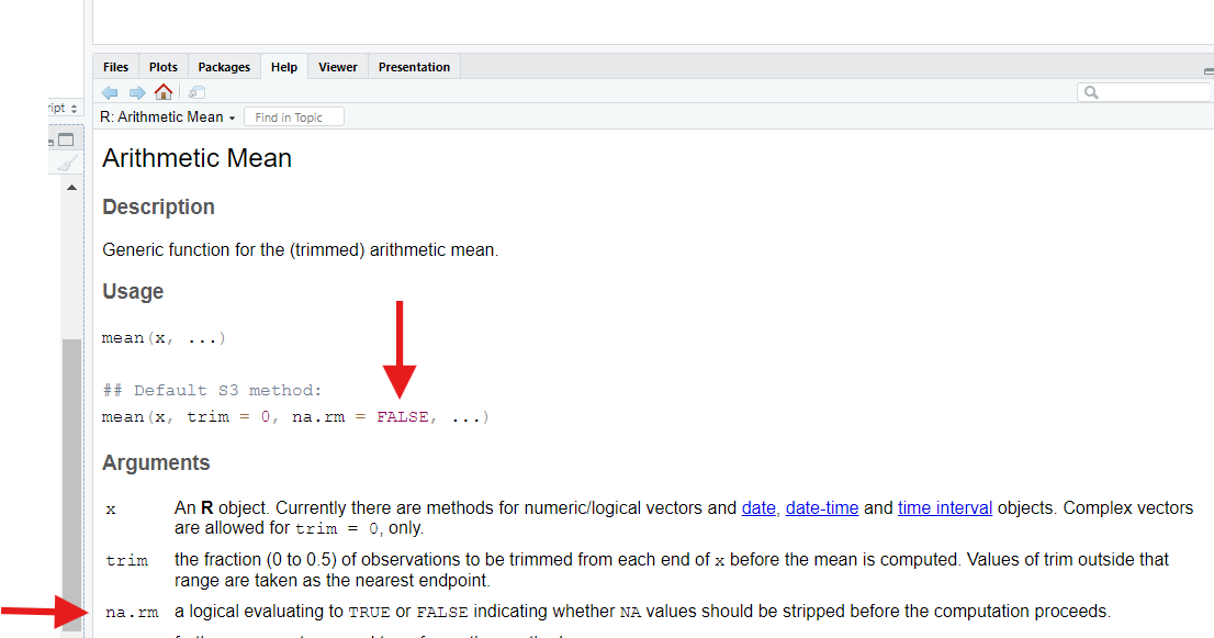
up mean()’s help page:
R
?mean
When we do, we discover that mean() has an optional
input, na.rm, that defaults to FALSE, which
means “don’t remove (rm) NAs when going to calculate a
mean.”
If we set this parameter to TRUE, mean()
will do what we want—it will strip out NAs before
trying calculating the average.
Challenge
However, if we try to do that like this, we get an error:
R
mean(testVector, TRUE)
Why doesn’t that command work?
We get an error that discusses trim. What even is
that?!
If we re-consult the function’s help page, we might discover that,
actually, mean() has three input slots, and
na.rm is the third one; the second one is
named trim.
Because we only provided two inputs to mean(), R assumed
we wanted those two inputs to go into the first two input
slots. So, we provided our na.rm input to the
trim parameter by mistake!
To avoid this, we could provide a suitable value for
trim also, such as it’s default value of 0,
like this:
R
mean(testVector, 0, TRUE)
This works, but we could also just match up our inputs with their target slots using the slots’ names, as we learned to do earlier:
R
mean(x = testVector, na.rm = TRUE)
Doing this allows us to skip over trim entirely (since
it’s an optional input)! That makes this approach easier.
Callout
This is another good reason to always name your function inputs. Some functions have dozens of input slots. If you only want to engage with the last few, e.g., using the parameter names to match up your inputs with those slots is the only sensible option!
Sequences
One thing regular R users find themselves needing to make surprisingly often is a sequence, which is a vector containing values in a specific pattern.
If we just want a simple sequence, from some number
to some number counting by one, we can use the :
operator:
R
-3:7
OUTPUT
[1] -3 -2 -1 0 1 2 3 4 5 6 7If we want to repeat a value multiple times, we can use the
rep() function:
R
rep(x = 3, times = 5)
OUTPUT
[1] 3 3 3 3 3rep() can also be used to repeat entire vectors of
values:
R
rep(x = -3:7, times = 5)
OUTPUT
 [1] -3 -2 -1  0  1  2  3  4  5  6  7 -3 -2 -1  0  1  2  3  4  5  6  7 -3 -2 -1
[26]  0  1  2  3  4  5  6  7 -3 -2 -1  0  1  2  3  4  5  6  7 -3 -2 -1  0  1  2
[51]  3  4  5  6  7
If we want to create a more complicated sequence, we can use the
seq() function:
Challenge
Both rep() and seq() have interesting
optional parameters to play with!
For example, what happens if you provide a vector (such as
c(1, 5)) to rep() for x? What
happens if you swap each in for times in the
command rep(x = -3:7, times = 5)? What happens if you swap
length.out in for by in the command
seq(from = 8, to = 438, by = 52)? Try it and see!
If we switch to each instead of times, we
instead repeat each value inside our vector that many times
before moving on to the next value:
R
rep(x = c(1,5), each = 5)
OUTPUT
[1] 1 1 1 1 1 5 5 5 5 5For seq(), when we specify a by, we are
telling R how large the step length should be between each new entry.
When our next entry would go past our to value, R stops
making new entries.
When we switch to using length.out, we tell R to instead
divide the gap between our from and our to
into that many slices and find the exact values needed to
divide up that gap evenly:
R
seq(from = 100, to = 150, length.out = 12)
OUTPUT
 [1] 100.0000 104.5455 109.0909 113.6364 118.1818 122.7273 127.2727 131.8182
 [9] 136.3636 140.9091 145.4545 150.0000
This results in an equally spaced sequence, but the numbers may be
decimals. Using by, however, may cause our last interval to
be shorter than all others, if we hit our to value before
we hit our by value again.
Logical tests
Just like a human language, R has question sentences. We call such commands logical tests (or logical comparisons). For example, run:
R
x = 5 # Create x and set its value
x == 5 #Is x *exactly* equal to 5?
OUTPUT
[1] TRUEAbove, we create an object called x and set its value to
5. We then ask R, using the logical
operator ==, if x is “exactly equal”
to 5? It responds with yes (TRUE), which we
know is correct.
[Yes, this a third, distinct use for the = symbol in R
(although, here, we have to use two; one won’t
work!).]
There are other logical operators we can use to ask different or more complicated questions. Let’s create a more interesting object to use them on:
R
logicVec = c(-100, 0.1, 0, 50.5, 2000)
Challenge
Then, try each of the commands below, one at a time. Based on the answers you receive, what questions do you think we’ve asked?
R
logicVec != 0
logicVec > 0.1
logicVec <= 50.5
logicVec %in% c(-100, 2000)
First, let’s see the answers we receive:
R
logicVec != 0
OUTPUT
[1] TRUE TRUE FALSE TRUE TRUER
logicVec > 0.1
OUTPUT
[1] FALSE FALSE FALSE TRUE TRUER
logicVec <= 50.5
OUTPUT
[1] TRUE TRUE TRUE TRUE FALSER
logicVec %in% c(-100, 2000)
OUTPUT
[1] TRUE FALSE FALSE FALSE TRUEAs you can see, logical tests are vectorized, meaning we compare each entry in our vector separately to the value(s) provided in the question, to the right of the logical operator.
For the first test of logicVec != 0, we get back only
one FALSE, for the third entry. Why? Well, that’s the only
entry whose value is exactly 0. If == is the
logical operator for “is equal to,” !=
must be the logical operator for “is not equal
to.”
For the second test of logicVec > 0.1, we get back
four TRUEs. This one hopefully makes intuitive sense; we’ve
asked which values are strictly greater than 0.1,
and since all but -100 are, we get four “yeses.”
For the third test of logicVec <= 50.5, we get back
four “yeses” as well because four values are either less than
(<) or equal to (=) a value of
50.5.
As you might guess, < and >= are also
logical operators; we just didn’t use them in these
examples!
The last example is a bit weirder. The %in%
logical operator is also called the match
operator. It asks “is each thing on the left also found in the
thing on the right?” That is, it is looking for matches between the left
and right inputs and, when it finds a match, we get TRUE.
“Is each thing on the left equal to anything on the
right?”
Here, we get back two matches, for the first and last entries in
logicVec, which makes sense because -100 and
2000 are indeed found in both vectors we’ve provided.
We can also ask R “multi-part” questions. For example, type and run the following:
R
logicVec > 0 & logicVec < 50
The & operator is the “and” logical
operator. So, here, we’ve asked R two questions that
must both be true for a value to get back a “yes.” Only two of our five
entries satisfy both questions we’ve posed, so we get back two
TRUEs.
Note that both questions need to be complete commands! You
can’t write, for example, just
logicVec > 0 & < 50, even though this would seem
both sensible and tempting.
Also, note that there is an operator for “or”: |. That’s
the “pipe” character, located over by your enter/return key. If you
connect two logical tests with |, so long
as either test passes for an entry, that entry will return
TRUE.
It may not be immediately clear what logical tests are good for, but we’ll see several use cases for them in later lessons.
Subsetting and indexing
We’ve seen both 1D (vectors) and 2D (matrices and data frames) objects, which contain more than one value and might contain millions! If these objects are big enough, printing them to the Console to see their contents would be impractical. How can we carefully and targetedly “look inside” an object?
We can use indexing. This is using a label (e.g., a column name) or index value (e.g., a row number) to “target” a specific value (or multiple values) inside an object.
For example, if we want to see just the first value inside
of the logicVec vector we built earlier, we could do
this:
R
logicVec[1]
OUTPUT
[1] -100The indexing operators, the square brackets [ ], are
keys you might not often use. If it helps you to remember what they’re
for, remember that they look like little “iron sights” you use to “aim”
at specific entries inside objects!
In the command above, we placed the index value 1 inside
our brackets and attached those brackets to the object we wanted to peer
inside.
An index value of 1 will ask R to retrieve the first
value. Logically, if we used an index value of 4 instead,
we’d get back the fourth entry:
R
logicVec[4]
OUTPUT
[1] 50.5Challenge
What happens if we use index values that make less sense? What if we ask for the 8th value, even there is no 8th entry? What if we ask for the “0th” entry? What if we ask for a “negative” entry? Run the following commands to find out:
R
logicVec[8]
OUTPUT
[1] NAR
logicVec[0]
OUTPUT
numeric(0)R
logicVec[-3]
OUTPUT
[1] -100.0 0.1 50.5 2000.0Each of these commands teaches us something different about how indexing works in R.
In the first, we ask for a non-existent 8th entry. R does
not respond with an error or
warning, as we might expect. Instead, it responds
NA. Essentially, it responds as though an 8th entry
could exist; it just doesn’t know what it’s value
would be because that value is currently missing (which could
technically be true). We mentioned earlier that many operations
produce NAs; this is one.
In the second command, we ask for a non-sensical “0th” entry. Again,
R does not respond with an error or warning. Instead, it
responds with a strange value: numeric(0). This is R’s way
of saying “your result is a numeric vector with 0
contents.” Uh…sure!
What’s important here is that this command proves R is different than many other programming languages. In Python, for example, asking for the zeroth entry is actually how you ask for the first entry—Python is a zero-indexed language, which means it starts counting positions at 0 instead of at 1. Row 0 is the first row!
Meanwhile, R is a one-indexed language—if you want the first
row or entry, you use an index value of 1, not
0. Even though that’s probably more intuitive, R is
actually uncommon; most common languages are zero-indexed.
In the third command, we ask for the “negative third entry.” We get
back every entry but the third. That’s because the
- operator, when used in indexing, excludes values at
certain positions rather than targeting them.
You can also use sequences as index values, if you want to peek at multiple values inside an object. Run the following commands to see two examples:
R
logicVec[2:4] #2nd thru 4th values
OUTPUT
[1] 0.1 0.0 50.5R
logicVec[c(1, 5)] #The first and fifth value.
OUTPUT
[1] -100 2000Indexing allows us to peek at specific values inside an object; what if we don’t like the values we see when we do that?
For example, in the testVector object we made earlier,
the fourth entry is NA, which caused problems. We can
combine indexing with assignment to
overwrite (replace) values inside objects. Here’s how
we’d replace that NA with 100:
R
testVector[4] = 100 #Replace the 4th value in testVector with 100.
testVector
OUTPUT
[1] 1 8 10 100If you provide an equal number of replacement values, you can replace multiple values at once:
R
testVector[c(2,4)] = c(-5, 32) #If indexing two values, must provide two replacements.
testVector
OUTPUT
[1] 1 -5 10 32What if we want to have a smaller object than the one we currently
have? We can also combine indexing and
assignment to create subsets (smaller
versions) of an object. Here’s how we’d create a new object containing
just the first and third entries of logicVec:
R
newVec = logicVec[c(1,3)]
newVec
OUTPUT
[1] -100 0This is how indexing works for vectors. It works a little differently with 2D objects. Let’s create a matrix and a data frame to experiment with:
R
mat1 = matrix(4:-4, ncol=3)
df1 = data.frame(x = 1:5, y = letters[1:5])
mat1
OUTPUT
     [,1] [,2] [,3]
[1,]    4    1   -2
[2,]    3    0   -3
[3,]    2   -1   -4
R
df1
OUTPUT
  x y
1 1 a
2 2 b
3 3 c
4 4 d
5 5 e
For vectors, our index values were the positions of the entries we were interested in (position 1, position 2, etc.). Single values make less sense for a 2D object—what’s the 6th position in a 3x3 matrix, for example? Is it the value in the 2nd row and 3rd column? In the 3rd row and 2nd column? Something else? Let’s see what R thinks:
R
mat1[6]
OUTPUT
[1] -1-1 is the value in the 3rd row and 2nd column. Is that
the value you’d have picked? This shows us that R reads (and fills)
matrices top to bottom and then left to right (unlike how
English speakers would probably read them).
Since that’s maybe confusing, it’d be easier to use two position values to index a matrix, one for the row number(s) we’re interested in and one for the column number(s) we’re interested in. We can separate these values inside our brackets using a comma, just like we do with inputs inside a function call.
For example, here’s how we’d get back the value from the 2nd row and 3rd column instead:
R
mat1[2, 3] #Second row, third column
OUTPUT
[1] -3When indexing using two index values like this, you always provide row information first and column information second. It’s just like in the game “Battleship,” in which you guess spots on a grid by saying their row identifier first.
What if we wanted back an entire row or column? We could do something like this:
R
mat1[1:3, 2] #The whole second column
OUTPUT
[1] 1 0 -1This works, but there’s an easier way. If we use a comma to create a slot, but we leave that slot blank, R interprets that blank slot as “give back all of these.” For example, if we run this command:
R
mat1[ , 2]
OUTPUT
[1] 1 0 -1We also get back the whole second column. By leaving the slot for rows blank, we’re telling R we want back all available rows.
Indexing works mostly the same way for data frames as it does for matrices, but there are a couple notable differences. For example, consider this command:
R
df1[2]
OUTPUT
  y
1 a
2 b
3 c
4 d
5 e
This command returns the entire second column of our data frame instead of giving us just the second value in it, like it would have for a matrix. This is because data frames are designed to hold data sets, and columns play a really important row in working with data sets, so R “favors” columns when indexing data frames.
Another sign of this is the existence of the $ operator.
We can use $ to index columns of a data frame by their
names instead of their positions:
R
df1$y #Whole y column
OUTPUT
[1] "a" "b" "c" "d" "e"This “shortcut” doesn’t work on matrices, even ones with named columns.
Notice how the two commands we’ve just run produce different-looking outputs—the first produces a data frame as an output, while the second produces a vector. This is a good example of how there are often multiple ways in R to produce similar (but also distinct) results.
We can index/subset objects using logical tests too.
For example, the following command would return only rows with values in
column 3 of our matrix that are greater than -4:
R
mat1[mat1[,3] > -4, ]
OUTPUT
     [,1] [,2] [,3]
[1,]    4    1   -2
[2,]    3    0   -3
This is another nested command, so
let’s break it down. Because R reads these from the inside out, we will
too. We’ve first asked R to determine which values in the third
column of mat1 are greater than -4:
R
mat1[,3] > -4 #The inside command above
OUTPUT
[1] TRUE TRUE FALSEWe get TRUE for the first two values and FALSE for the last value.
Then, we ask R to only keep rows in mat1 that
are TRUE and exclude all rows that are FALSE, according to
that rule (and we keep all columns by leaving the column slot
blank):
R
mat1[c(TRUE, TRUE, FALSE), ] #Basically what we did.
OUTPUT
     [,1] [,2] [,3]
[1,]    4    1   -2
[2,]    3    0   -3
In this way, we’ve created a subset of our matrix that passes a test
we care about—something we often want to do with our data sets!
We’ll see even fancier ways to create subsets like this when we learn
the dplyr package later. Speaking of which…
Installing and loading packages
Much earlier on, we noted there are thousands of add-on packages for R. Because there are so many, it makes sense R does not come installed with all these. That would be a lot of files!
So, if we want to use these other packages (and we do), we’ll have to download and install them first. This is, thankfully, easy ( assuming we know the name of the package we want).
In a later lesson, for example, we’ll use the dplyr
(pronounced “Dee-Plier”, or “Dee-Ply-Ar”, or “Dipply-Er”) package, which
contains an amazing set of tools for cleaning and manipulating
data sets; many R users use dplyr’s tools every
day. Let’s use dplyr as our example package here.
First, we have to download and install dplyr; the
following command will do that:
R
install.packages("dplyr")
In just a few moments, you should get confirmation that
dplyr has installed (assuming you have an internet
connection!).
However, by default, R does not assume you want to actually use all the packages you have installed. Thinking back to our “room” analogy, if we had hundreds of packages on, each one full of tools and other stuff, dumping all that stuff into our “room” would make it very cluttered!
So, every time we start R, we have to manually turn on
any packages we want to use. To do this, we use the
library() function:
R
library(dplyr)
This will turn on dplyr and make all its tools and stuff
accessible.
Note we needed to quote "dplyr" in
install.packages(), but we didn’t need to in
library(). There’s not really a good reason for this—to
some degree, you have to memorize when quotes are needed (or check help
pages).
Later, if we we want to turn a package off, we can use the
detach() function:
R
detach(dplyr)
We can also check to see if packages are already on/off, install or update packages, or turn packages on/off on the Packages pane, typically found in the lower-right (though it could be elsewhere):
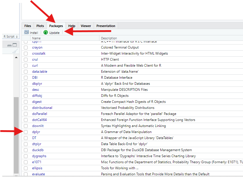
Here, you can use the “Install” and “Update” buttons at the top to install or update packages. In the table, meanwhile, you’ll find an alphabetized list of every package you have installed. If the checkbox next to a package’s name is checked, that package is on. Checking the checkbox will turn the package on; unchecking it will turn it off.
Many beginners find the Packages pane to be an easier way to deal with packages than using function calls.
Callout
Note that while you have to turn packages on every time you open R,
you only have to install a package once! For this
reason, don’t include install.package()calls in
your scripts; they are almost always unnecessary, and sometimes,
they take a long time to run!
Challenge
To practice managing packages, download and install the other
packages we’ll need for these lessons: gapminder,
ggplot2, and tidyr. Then, turn them on.
First, you’d use install.packages() to download and
install each package. We can actually put all the packages into a single
call if we want, so long as we separate them with commas. We also have
to quote each package name:
R
install.packages("gapminder", "ggplot2", "tidyr")
Then, we use library() to turn each package on. Unlike
with installation, we don’t have to quote the package
names, but we also can’t stuff all the packages into a single
call either, so turning on multiple packages is
tedious:
R
library(gapminder)
library(ggplot2)
library(tidyr)
We could just as easily do all this with the Packages pane instead, but that’d be harder to show here.
Managing your working directory
In the next section (the last in this lesson), we’ll talk about loading files into R and saving files from R. Those are things you’ll probably do often if you use R regularly!
Before that, though, we need to explain a quirky R concept: your working directory.
When you start R, R assumes that, for that session, there is a “home base” on your computer it should interact with. This “home base” is called your working directory (a “directory” is another name for a “folder”).
To figure out what your working directory is, use
the getwd() function:
R
getwd()
We can also figure out our working directory by clicking the “right arrow” at the top of the Console:
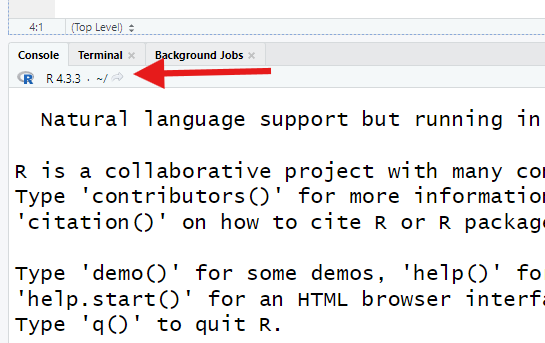
This opens our working directory in the Files pane, typically found in the bottom-right (though it could be elsewhere).
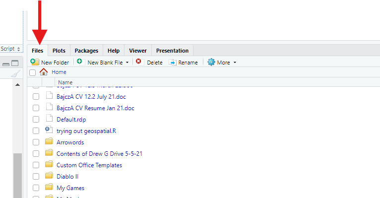
If we try to load a file into R, unless we specify otherwise, R assumes it’s in our working directory. If we save a file from R, unless we specify otherwise, R assumes it should save it into our working directory. So, it matters which folder this is!
If we want to change our working directory,
we can specify a new directory by providing a file
path to the setwd() function:
R
setwd("some/path/to/a/different_folder")
However, for beginners, file paths can be tricky, so thankfully there’s an easier way. Find “Session” at the top of your screen. There, select “Set Working Directory.” Then, click “Choose Directory…”. This’ll bring up a “file picker” on your computer, allowing you to navigate to the folder you want to choose. Much easier!
Loading and saving files
How exactly you load or save files in R depends on what exactly you are trying to load or save, understandably!
However, in general, you will use a read
function of some kind to load files. For example,
read.csv() will read data a .csv (“comma-separated values”)
file, readRDS() will read an .rds (“R data structure”)
format, and so on. Other packages add additional options; for example,
the readxl package adds the read_excel()
function for loading Microsoft Excel files.
To demonstrate how to load files into R, we need a file to load. So, let’s first make an object we can save to demonstrate how saving works. Run:
R
#Thoughtfully placed line breaks can help us see the separations between inputs in our function calls!
sampleData = data.frame(x = c(1, 2, 3),
                        y = c("A", "B", "C"))
This command creates a data frame with two columns
(named x and y), each with three values, so
the result has three rows. [Sidenote: We have yet another,
distinct use of = here! Here, we’re using it to give
names to the columns we’re creating. This is its job
insidecertain functions, like data.frame.]
Now, we can save this data frame as a simple .csv file using
write.csv(), which has two required inputs:
The R object we want to save, and
The name we want to give the file, which should end in “.csv”. This input must be quoted.
So, run:
R
write.csv(x = sampleData,
          file = "sample.csv")
So long as that command worked, you should see your new file in your Files pane (you may need to “Refresh” the pane first using the circular arrow button in the pane’s top-right corner).
Now that we have that file, we can read it into R using
read.csv(), which takes just one required input: the name
(or path) of the file we’re loading. However, to actually make the data
set we’re loading permanent, we need to combine it with an assignment
command to give the new object a name as well:
R
sample_data = read.csv("sample.csv")
In other words, we almost always pair a read function
with an assignment command to save what we’re reading
as a named object so R won’t forget it as soon as it’s
done reading it.
RStudio offers a second way to load data that some may find easier, though it’s harder to explain here. In your Environment pane, find the “Import Dataset” button, then select the appropriate option for the format of data you want to import.
A large window will then open:
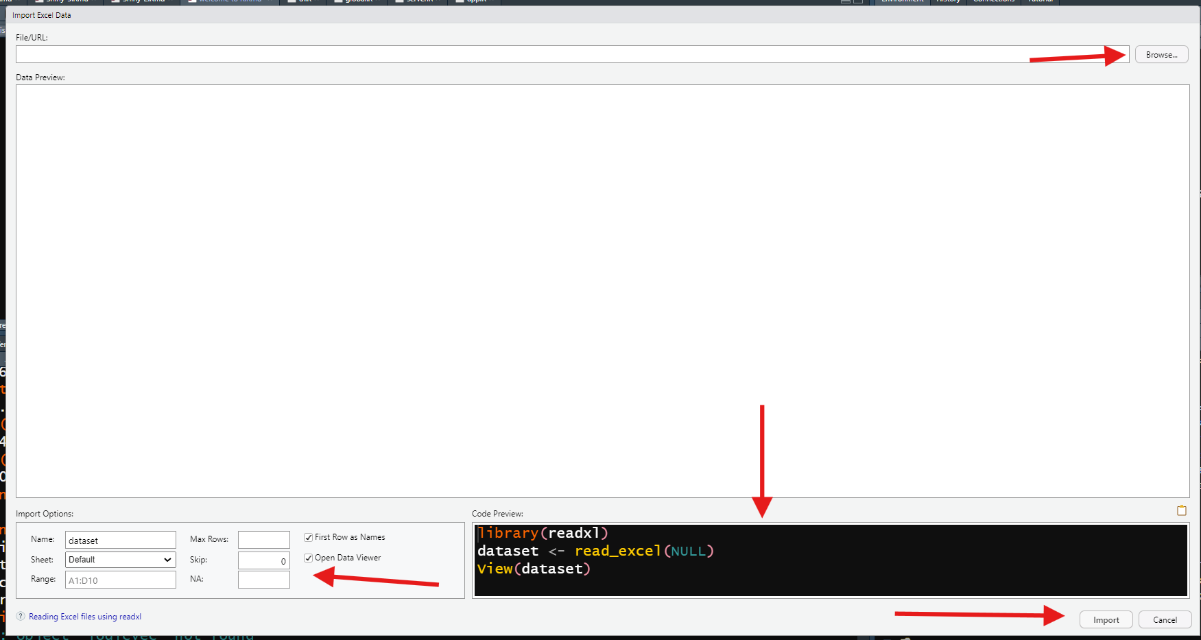
This window allows you to select the file you want to load using a file picker (towards the top). A preview of the data you’ve loaded is then provided in the center.
At the bottom-left, you’ll see options to adjust which rows to import and whether the top row should be treated as column names. You can also name your new data set object here. If you’re curious, the code needed to achieve the same outcome is displayed in the bottom-right. When you’re satisfied, hit the “Import” button.
Creating an R Project folder
We’ve seen that, when working in R, managing your environment is important, managing your working directory is important, and loading and saving files is important. All these are made easier by having an R Project folder.
When you make one, R adds a .rproj file to a folder on your computer. When you then launch R by opening this .rproj file, or when you use the “File” menu to open this file or project, R will use the contents of this .rproj file to restore your environment, package statuses, and open files to whatever they were the last time you worked on your project.
This means that, for large or complicated projects, you can “save your progress” between R sessions! Furthermore, R will assume your working directory is your project folder, which means saving and loading project files is easier (assuming you store them in your project folder, of course)!
To make an R Project folder, go to “File,” then select “New Project.” A menu will pop up; there, select “New Directory,” then select “New Project.”
On the next screen, use the file picker to select a location for your new project folder on your computer, then give it a name. Also, check the box that says “Open in New Session.” When you’re ready, press “Create Project.” This will open a new session of RStudio centered around your new Project.
Key Points
- R is an incredibly powerful tool; knowing how to use it is an incredibly valuable skill. However, to learn it takes the same diligence as learning a human language does.
- R is a very capable calculator; you can use it to do math.
- R, like human languages, has punctuation marks (operators) that have specific meanings and usage rules.
- R “sentences” are called commands. They include inputs as well as instructions for operations we want R to perform for us.
- Script files are text files that allow us to write and store code and annotations and then “teleport” this code to the Console when we’re ready.
- “Nouns” in R are called objects. These are impermanent until we use assignment commands to name them, in which case they persist until we overwrite them or close R.
- Our environment is everything we have named since starting our R session.
- There are rules about what we can and can’t (and should and shouldn’t) name objects in R.
- R is case-sensitive, so capital and lowercase letters are distinct.
- It’s good to have a naming convention to name objects.
- Objects in R take many different shapes, and the values they store can be of many different types (the “adjectives” of the R language).
- In R, “verbs” are called functions. Functions take inputs, perform operations, and produce outputs. Some functions do math; others might create new objects.
- Functions have slots for specific inputs. These slots are called parameters, and they have names. The inputs we provide to these slots are called arguments. Arguments should be given in a specific order, and they should be of specific types.
- Some function inputs are optional; others are required. Optional inputs are like R’s “adverbs” in that they often control how R performs a specific operation.
- If we want help with a function, we can use the
?operator to open its help page. - The
=symbol has many different uses in R, which can be confusing. As such, consider using<-for assignment. - Logical tests are like “questions” in R. There are many different logical operators to ask a variety of questions.
- Use the square bracket operators
[ ]to peek inside objects in indexing commands. Indexing commands can also be used to update or subset objects, and their format differs for 1D vs. 2D object types. - Installing packages is necessary to have access to them, but even then, packages must be turned on to use their features.
- Your working directory is the folder R assumes it should interact with on your computer when loading/saving files.
- R Project folders are handy for keeping organized when working on a large, important, or complex project.
- Loading files in R typically requires a
readfunction; saving files typically requires awritefunction.